Joins are a crucial transformation when it comes to data. It allows us to enrich the data that we currently have with some more data. As the name suggests, the join() method allows us to join two dataframes. We are allowed to define what strategy is to be used and on what conditions the dataframes are to be joined. I had given a brief introduction in this article, if you have not checked it out I kindly request you to do so.
The join() method takes three arguments:
other
on
how
The other should be an object of Class DataFrame, argument on should be either a condition or a list of column(s) or column name(s). Argument how determines what join strategy is to be used.
The how argument accepts a variety of string values that should be one of the following:


inner:
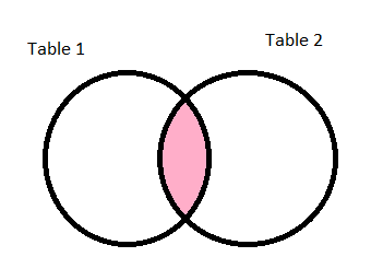
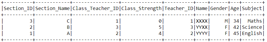
The inner value is the default for the how argument. The final dataframe consists only of rows that satisfy the join condition. If we want the join to be an inner join, it is not necessary to pass the value as depicted in the example:
# not passing inner as an argument
df_sections.join(df_teachers,
df_teachers.Teacher_ID == df_sections.Class_Teacher_ID).show()
# passing inner as a argument
df_sections.join(df_teachers,
df_teachers.Teacher_ID == df_sections.Class_Teacher_ID,'inner').show()
outer
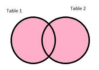
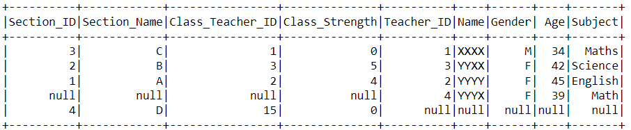
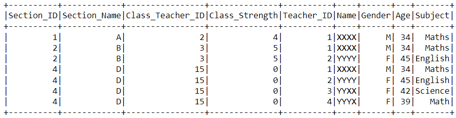
The outer value is used to perform a full outer join. The final dataframe will consist of records from both of the dataframes, the count of the resulting dataframe will be the count of the biggest dataframe out of the two. For rows that do not satisfy the join condition, the columns from the other dataframe are populated with a null. As in the below case where Teacher_ID 4 does not satisfy the join condition and the columns from the Section dataframe for that row are filled with nulls. A similar scenario can be observed for the row with Section_ID 4. As indicated in the table, this type of join can be performed using four different how values: outer, full, fullouter, full_outer:
## using outer
df_sections.join(df_teachers,
df_teachers.Teacher_ID == df_sections.Class_Teacher_ID, 'outer').show()
## using full
df_sections.join(df_teachers,
df_teachers.Teacher_ID == df_sections.Class_Teacher_ID, 'full').show()
## using fullouter
df_sections.join(df_teachers,
df_teachers.Teacher_ID == df_sections.Class_Teacher_ID, 'fullouter').show()
## using full_outer
df_sections.join(df_teachers,
df_teachers.Teacher_ID == df_sections.Class_Teacher_ID, 'full_outer').show()
left
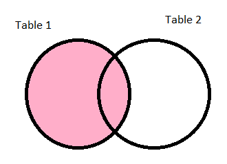
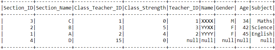
The value left is used when we want to perform a left outer join. The resulting dataframe will have all the records from the left hand side dataframe, irrespective of whether they satisfy the condition or not. So the record count of the result will always be the count of the dataframe in the left side of the join. If we have selected columns from the right hand side dataframe, for the left hand side dataframe rows that did not satisfy the join condition these columns will be filled with null. This is depicted by the join result below, the Class_Teacher_ID 15 did not find any match on the df_teachers, hence the columns from the df_teachers are filled with null. We can instruct Spark to perform left outer join using three different values for how: left, leftouter, left_outer.
## using left
df_sections.join(df_teachers,
df_teachers.Teacher_ID == df_sections.Class_Teacher_ID, 'left').show()
## using leftouter
df_sections.join(df_teachers,
df_teachers.Teacher_ID == df_sections.Class_Teacher_ID, 'leftouter').show()
## left_outer
df_sections.join(df_teachers,
df_teachers.Teacher_ID == df_sections.Class_Teacher_ID, 'left_outer').show()
right
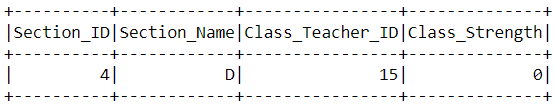
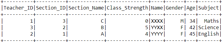
The value right is commonly used when we want to perform a right outer join. The resulting dataframe will have all the records from the right hand side dataframe, hence the count of the resulting dataframe will be the count of the dataframe on the right side of the join. If we have selected any columns from the left hand side dataframe, for the right hand side dataframe rows that do not satisfy the join condition, the value of these columns will be set to null. This is clearly depicted by the row which has Teacher_ID as 4, the columns of the df_sections are set to null as there was no match of Teacher IDs. We can instruct Spark to perform right outer join by passing one of the three values for the how argument: right, right_outer, rightouter.
## using right
df_sections.join(df_teachers,
df_teachers.Teacher_ID == df_sections.Class_Teacher_ID, 'right').show()
## using rightouter
df_sections.join(df_teachers,
df_teachers.Teacher_ID == df_sections.Class_Teacher_ID, 'rightouter').show()
## using right_outer
df_sections.join(df_teachers,
df_teachers.Teacher_ID == df_sections.Class_Teacher_ID, 'right_outer').show()

semi
The value semi is commonly used when we want to perform a left semi join. This type of join is very similar to inner join with respect to rows that are returned(only the rows that satisfy the join condition), but the resulting dataframe will only have the columns from the left hand side dataframe. This can be easily achieved without using semi join, by including a select statement after a normal inner join. But using semi join is much more efficient than taking the long alternative. The count of the result will depend on how many rows satisfy the join condition. Since this type of join is partly inner and no columns of the right hand side dataframe will be present in the result,Spark will not automatically fill these columns with null for any row. We can instruct Spark to perform a semi left join by passing one of the three possible values for the how argument: semi, leftsemi, left_semi
# using semi
df_sections.join(df_teachers,
df_teachers.Teacher_ID == df_sections.Class_Teacher_ID, 'semi').show()
# using leftsemi
df_sections.join(df_teachers,
df_teachers.Teacher_ID == df_sections.Class_Teacher_ID, 'leftsemi').show()
# using left_semi
df_sections.join(df_teachers,
df_teachers.Teacher_ID == df_sections.Class_Teacher_ID, 'left_semi').show()
# using an inner join in combination with a select statement
df_sections.join(df_teachers,
df_teachers.Teacher_ID == df_sections.Class_Teacher_ID)
.select(*df_sections.columns).show()
Unpacking df_sections.columns has saved me from typing out all the column names, learning the utility functions and attributes of dataframes can help us save much of our time.

anti
The value anti is commonly used as an argument when we want to perform left anti join. The resulting dataframe will contain records from the dataframe on the left side of the join, which did not satisfy the join condition. The result will not contain any columns from the dataframe on the right side of the join. The total count of records depends on how many rows do not satisfy the join condition from the left. We do have an alternative way to achieve the same results with the help of a left outer join, post which a where condition and a select usage. But as mentioned in the case of semi join, using the anti value for the how argument is much more efficient. We can use three possible values for the how argument: anti, left_anti, leftanti.
# anti
df_sections.join(df_teachers,
df_teachers.Teacher_ID == df_sections.Class_Teacher_ID, 'anti').show()
# left_anti
df_sections.join(df_teachers,
df_teachers.Teacher_ID == df_sections.Class_Teacher_ID, 'left_anti').show()
# leftanti
df_sections.join(df_teachers,
df_teachers.Teacher_ID == df_sections.Class_Teacher_ID, 'leftanti').show()
# using the alternative
df_sections.join(df_teachers,
df_teachers.Teacher_ID == df_sections.Class_Teacher_ID, 'left')
.where(df_teachers.Teacher_ID.isNull()).select(*df_sections.columns).show()
cross
The cross join is not the most common type of join in data transformation. It is usually used to create data that did not exist before, from some existing data. The cross join, as you might already be aware, is cartesian product of two data sources. cross value can be passed to how, in order to perform cross join. The count of the resulting dataframe will be the product of counts of both of the dataframes involved in the join.
We can also use an alternate method provided with the dataframe to achieve the same result. The method is crossJoin(). I did not cover this method in the Dataframes 101 series because it is more appropriate to discuss the method in the context of joins. This method is much more intuitive than the join method (especially for cross join). The method takes only one argument, which is another dataframe. For cross join, if we do not have any condition crossJoin() can be used. But if we have a join condition, like in the following example, we only have the option of using the normal join() method.
roll_1 = spark.range(1,7).select(col('id').alias('Face1'))
roll_2 = spark.range(1,7).select(col('id').alias('Face2'))
# using a special method called crossJoin
roll_1.crossJoin(roll_2).show(5)
# using the join method’s how argument cross
roll_1.join(roll_2,
(roll_1.Face1.isNotNull() & roll_2.Face2.isNotNull()),'cross').show(5)

Since the result had 36 records(6 records from the left x 6 records from the right), I decided not to display the entire result. But you try using the same code to inspect the entire result.
Argument ‘on’
We have a lot of options when it comes to specifying the join condition using the on argument. The first way is to provide a Column expression:
expr('Class_Teacher_ID = Teacher_ID')
(or)
col('Class_Teacher_ID') == col('Teacher_ID')
(or)
df_sections.Class_Teacher_ID == df_teachers.Teacher_ID
All the expressions above mean the same and these expressions will help us perform equi-join(join based on equality of attributes). Using join(), we are not restricted to perform only equi-joins; some non-equi join conditions can be seen below. Even though these do not make much sense, it proof that non-equi joins work:
df_sections.join(df_teachers,
df_sections.Class_Teacher_ID > df_teachers.Teacher_ID).show()
The next type of argument that can be passed to the on argument is a string, which is a column name. This type is used only when we want to perform an equi-join based on identically named columns in both of the dataframes. To illustrate this case, I have made a small change in the column name Class_Teacher_ID in the df_sections.
data_sections = [[1,'A',2,4],[2,'B',3,5],[3,'C',1,0],[4,'D',15,0]]
data_teachers = [[1,'XXXX','M',34,'Maths'],[2,'YYYY','F',45,'English'],
[3,'YYXX','F',42,'Science'],[4,'YYYX','F',39,'Math']]
columns_teachers = ['Teacher_ID','Name','Gender','Age','Subject']
columns_sections = ['Section_ID','Section_Name','Teacher_ID','Class_Strength']
df_teachers = spark.createDataFrame(data_teachers,columns_teachers)
df_sections = spark.createDataFrame(data_sections,columns_sections)
I have changed the name of that column to Teacher_ID , which can also be found in the df_teachers. So in order to join these two tables, a method call as simple as the following is sufficient:
df_sections.join(df_teachers, 'Teacher_ID').show()
The result will have only one of the commonly named columns. Which dataframe’s, either the left or the right, column is retained depends on the type of the join. If the join is left, then the left dataframe’s column is retained in the result and the opposite applies for the right join.
The next type of value that can be passed is a list of strings, where each string is a column name. We can use this type of value when we want to perform an equi-join on multiple columns and these columns mentioned are present in both of the dataframes. To illustrate this use case, I have generated two new datasets, for which the source code is as follows:
data1 = [[1,1,'X'],[1,2,'X']]
data2 = [[1,1,1,'A'],[2,1,2,'B']]
columns1 = ['Section_ID', 'Roll_Num', 'Name']
columns2 = ['Parent_ID', 'Section_ID', 'Roll_Num', 'Parent_Name']
df1 = spark.createDataFrame(data1, columns1)
df2 = spark.createDataFrame(data2, columns2)
df1.show()
df2.show()
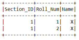
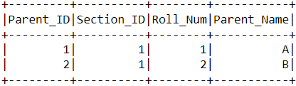
The first dataframe contains data for students, including details of their Section, Roll number and Name. The second dataframe consists of data for the parents, including details of their name and IDs(acts as a surrogate key) to identify their child’s record from the first dataframe. For the first dataframe, the primary key is Section_ID and Roll_Num together. So to join these two tables properly, we have to use the Primary key of the first dataframe on a equi-join as follows:
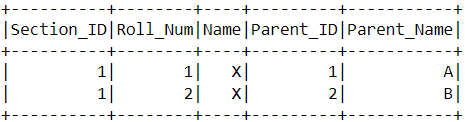
df1.join(df2, ['Section_ID', 'Roll_Num']).show()
In the last few examples only inner joins were depicted. But that does not mean the on argument’s value cannot be used in different types for other joins. All the value types apply to all the joins.
Conclusion
In this article I have covered join in full depth and this should be more than enough to work with joins in Spark. If you have any suggestions or questions please post it in the comment box. This article, very much like every article in this blog, will be updated based on comments and as I find better ways of explaining things. So kindly bookmark this page and checkout whenever you need some reference.
Comments
Post a Comment