Reading Delimited Files:
To read delimited files with Spark, the format method should be called with the argument “csv” even if the file that we are dealing with is not delimited by commas. That would inform spark that the files it is going to be dealing with are delimited files. Following are some of the examples of delimited file reading:
The following line reads a comma delimited file(s) inside path, specifies the first line of the file is a header and instructs spark to infer the schema. One important thing to keep in mind before using inferSchema is when spark is left to infer the schema, Spark creates a new job to read a large portion of the file to ascertain the schema. This can be really expensive, in terms of resources, for large files.
path = “...”
df = spark.read.format(“csv”).option(“header”,”true”)
.option(“inferSchema”,”true”)
.load(path)
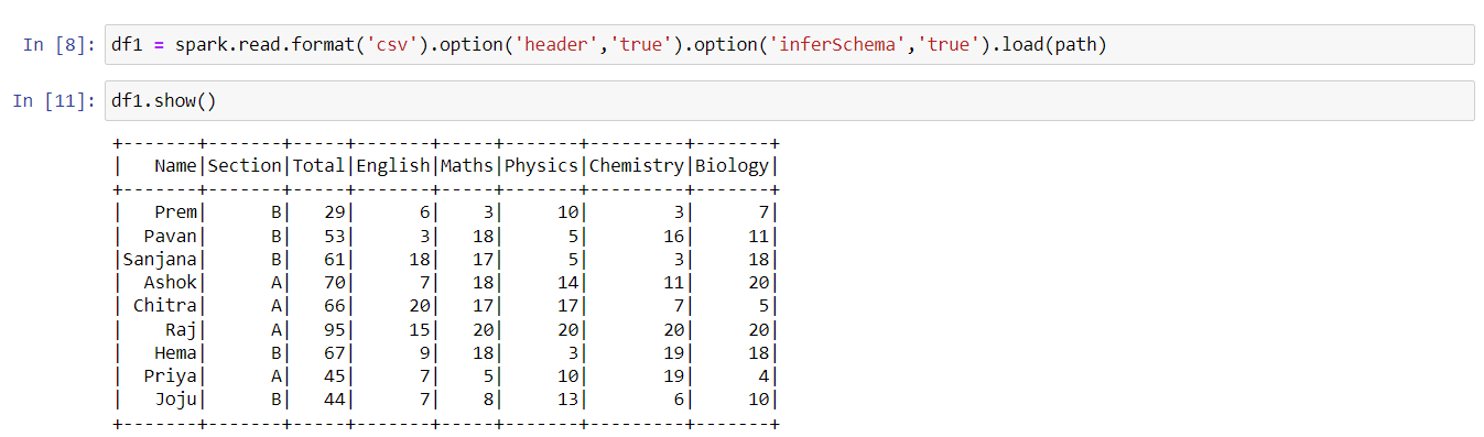
The following examples reads pipe delimited file(s),configured using the sep option, inside path, specifies the first line of the file is a header and instructs spark to infer the schema. They both achieve the same result mentioned above but the definition of configurations differ syntactically.
df = spark.read.format(“csv”).option(“header”,”true”)
.option(“sep”,”|”)
.option(“inferSchema”,”true”)
.load(path)
or
options_dict = {“header”:”true”,“sep”:”|”,“inferSchema”:”true”,”path”:path}
df = spark.read.format(“csv”).options(**options_dict)
.load()
The next examples read CSV files, but the schema is explicitly given.
schema = “““Name STRING,Section STRING,Total INT,
English INT,Maths INT,Physics INT,
Chemistry INT,Biology INT”””
df= spark.read.format('csv')
.schema(schema)
.option("header","true")
.load(path)
or
from pyspark.sql.types import *
schema = StructType([StructField("Name",StringType()),
StructField("Section",StringType()),
StructField("Total", IntegerType()),
StructField("English", IntegerType()),
StructField("Maths", IntegerType()),
StructField("Physics", IntegerType()),
StructField("Chemistry", IntegerType()),
StructField("Biology", IntegerType())])
df = spark.read.format('csv')
.schema(schema)
.option("header","true").load(path)
We can verify if the schema that we have has been applied while reading the files using:
df.printSchema()
O/P:
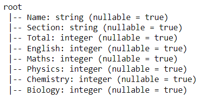
A very interesting characteristic of this schema is that Spark enforces the schema when reading the data. So the columns will be casted to the given type in schema. If we give a wrong type, for example if I try defining timestamp as the type for the Biology column:
schema = """Name STRING,Section STRING,Total INT,English INT,Maths INT,
Physics INT,Chemistry INT,Biology TIMESTAMP"""
df = spark.read.format('csv')
.schema(schema).option("header","true")
.load(path)
df.printSchema()
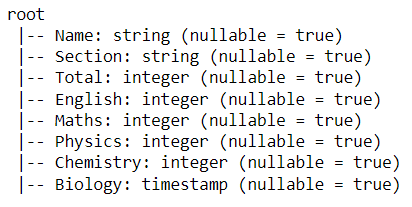
Spark does not throw any error and indeed casts the column to timestamp while reading the data. So when we try to view the column’s data:
df.select(‘Biology’).show()
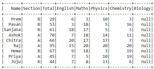
The values are null because the integers were casted to TimestampType. This is also due to the default read mode - permissive. We can do the following to view the _corrupt_records columns that will print out the entire record as seen in the file:
schema = StructType([StructField("Name",StringType()),
StructField("Section",StringType()),
StructField("Total", IntegerType()),
StructField("English", IntegerType()),
StructField("Maths", IntegerType()),
StructField("Physics", IntegerType()),
StructField("Chemistry", IntegerType()),
StructField("Biology", TimestampType()),
StructField('_corrupt_record',StringType())])
df = spark.read.format('csv')
.schema(schema).option("header","true")
.option("columnNameOfCorruptRecord", "_corrupt_record")
.load(path)
columnNameOfCorruptRecord option gives the column name that should consist of the deformed records. One way to instruct spark to avoid this behavior is to use the FAILFAST like in the following example:
df = spark.read.format('csv')
.schema(schema).option("header","true").option(“mode”,”FAILFAST”)
.load(path)
Which would result in an error like:

Writing Delimited Files:
To write delimited files with Spark, the format method should be called with the argument “csv” even if the file that we are dealing with is not delimited by commas. That would inform spark that the files it is going to be dealing with are delimited files. The header option is mandatory in all of the following examples because I want the header to be written as the first line of the files. Without this option the files will not have the header line. Following are some of the examples of delimited file writing:
df.write.format(‘csv’).option(‘header’,’true’).save(path)
The following example writes the dataframe’s content as CSV file(s). The number of files depends on the number of spark partitions in memory. But we can always choose to change the number of partitions. The repartitioning will be covered in another article.
df.write.format('csv').option('header','true')
.save(path)
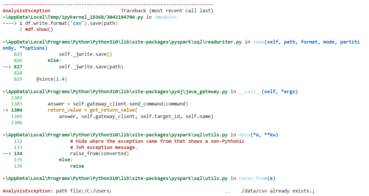
Since the default write mode is errorIfExists, the writing operation will fail because there are some files present in the given directory.
The following example writes the data into the same directory but the only difference is the write mode is overwrite. This will make sure that the data is written even if any files are found.
df.write.format('csv').option('header','true')
.mode('overwrite').save(path)
The following example depicts how to write data as pipe delimited files.
df.write.format('csv')
.mode('overwrite')
.option('header','true')
.option(‘sep’,’|’)
.save(path)
One of the common actions that is performed while writing to filesystems is partitioning with respect to one or more columns. Partitioning by column(s) creates folders for each unique value of the column(s) and the files inside the folder will contain only data for the corresponding column(s) value(s).Partitioning does not just make the data more easier for us to access but also provides Spark an option to perform predicate pushdown, but it does not apply to CSV files. This example depicts partitioning with the Section column and writing the CSV files.
df.write.format('csv').option('header','true')
.partitionBy('Section')
.mode('overwrite')
.save(path)
Resulting in:

In the following example, the path has not been changed and the only difference is the write mode. The files are appended to the respective Section directories, no files that are already present are affected:
df.write.format('csv')
.partitionBy('Section')
.option('header','true')
.mode('append').save(path)
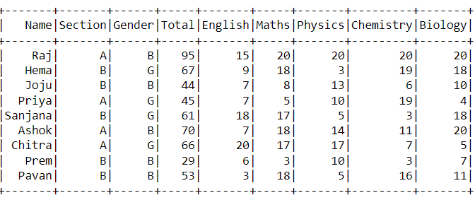
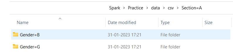
One more example with partition by multiple columns can be seen below(one more column “Gender” has been added):
df.write.format('csv')
.partitionBy('Section','Gender')
.option('header','true')
.mode('overwrite').save(path)
Which would result in:
Conclusion:
This article covered basic examples using the options that we have seen in th previous article. But all the options available in Spark are not covered for obvious reasons. I hope this was helpful and if you have any suggestions or questions please post it in the comment box. This article, very much like every article in this blog, will be updated based on comments and as I find better ways of explaining things. So kindly bookmark this page and checkout whenever you need some reference.
Happy Learning! 😀
Comments
Post a Comment