Spark Structured API execution can be split up into 3 high level steps:
The syntax of the code is checked (common for any code)
If the code is found to be valid, Spark converts this to a Logical Plan
This Logical plan is then converted to Physical plan. In this process, any optimizations that are possible are applied.
Spark executes this Physical Plan(RDD manipulations) on the cluster
The first step does not just apply to Spark but to all types of programs. Python checks for syntax of the code written, and fails the job if there is any violation of syntax. The second step is what I would describe as Spark-specific. In this step, a sequence of three types of Logical plans are created, with the most optimal one at the end. Logical plans are abstract, with no clarity on low-level execution details. We could imagine it to be similar to a flow chart that gives a high-level idea about how operations are to be performed and in what order. As the high-level is a good start, a detailed plan is required to actually do the job in a most efficient way. So for that reason spark converts this high level logical plan to a low-level physical plan, which has detailed information. For instance, the physical plan will clearly spell out where a particular task is to be performed in the cluster. Once this low-level plan is ready, Spark executes the job on the cluster. In the following sections, Logical and Physical plans are explained in depth. All these plans are created for each Spark Job.
Logical Plan:
The initial step of execution is meant to convert the user code to a logical plan(unresolved). The logical plan represents a set of abstract transformations without any reference of executors or drivers or any low level details. At the end of this first step the user's code will be converted to the most optimal logical plan. The formulation of an optimized logical plan involves a series of steps. As the first step in the journey,the driver generates an unresolved logical plan,after performing syntax checks. This plan is called an unresolved logical plan because the tables, columns and functions referenced in the code are not verified whether they are valid. In short, the plan is not yet validated.
Once the Unresolved Logical Plan is generated, the next step is to analyze the referenced tables, columns and functions. This step in the entire execution is called the Analysis. This analysis involves validation of the aforementioned entities with Spark's Catalog, the metadata store. This analysis is performed by a component called Analyzer. The Unresolved Logical Plan might get rejected if any of the entities referenced are not valid, due to which the job is failed. If the analyzer is able to verify, it emits a Resolved Logical Plan.
The Resolved Logical Plan is passed through a component called Catalyst Optimizer. Catalyst Optimizer is a programmatic optimizer built based on functional programming constructs in scala. The optimizer’s purpose, as the name suggests, is to optimize the logical plan. The catalyst optimizer creates an Optimized Logical Plan from the Resolved Logical Plan. This phase of execution is called Logical Optimization.
After successfully creating an Optimized Logical Plan, Spark then begins the physical planning process by generating a physical plan. This phase of execution is called the Physicall Planning. Physical plan specifies how the Logical Plan will execute on the cluster. In that process, the Catalyst optimizer generates multiple physical execution strategies. The physical plans are compared using a cost model. Each physical plan that is generated is assigned a cost and the one with the lowest cost is selected for execution.
The chosen Physical plan is used for low-level code generation with a series of RDDs and transformations. This final phase is called Code Generation. This phase involves generating efficient Java bytecode to run on every machine. Project Tungsten, which is a component of Spark, plays a role here. Because transformations in DataFrame,DataSet and SQL are converted into RDD transformations, from high level to low-level, Spark is popularly known as a compiler. It is important to note that plan generation is not a lazy process like transformations.
Spark allows us to inspect the execution plan for any dataframe, irrespective of whether the dataframe was created by a set of transformations on data from a source or managed table(using spark SQL). Dataframe comes with an explain method, which prints both the logical and physical plan. The method has the following syntax:
df.explain(extended=True/False, mode=mode)
Both of the arguments are optional. The extended argument is by default False and only prints the physical plan. If set to True, all of the logical plans are displayed with the physical plan. The mode argument can be used to format the output. Spark only allows specific set of values for this argument and they are as follows:
As you might have understood by now, both of the arguments to the explain method are used to format the output. mode argument provides much more control than the extended argument. The following examples illustrate how some of the mode values display the plans:
data = [('Raj','A','B',95,15,20,20,20,20),
('Hema','B','G',67,9, 18, 3, 19, 18),
('Joju','B','B',44,7,8,13,6,10),
('Priya','A','G',45,7,5,10,19,4),
('Sanjana','B','G',61,18,17,5,3,18),
('Ashok','A','B',70,7,18,14,11,20),
('Chitra','A','G',66,20,17,17,7,5),
('Prem','B','B',29,6,3,10,3,7),
('Pavan','B','B',53,3,18,5,16,11)]
columns = ['Name','Section','Gender','Total',
'English','Maths','Physics','Chemistry','Biology']
df = spark.createDataFrame(data,columns)
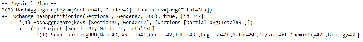
df.groupBy('Section', 'Gender').avg('Total').explain() # simple mode
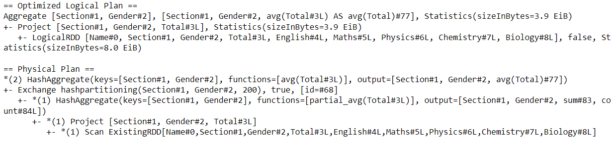
df.groupBy('Section', 'Gender')
.avg('Total').explain('cost') # involves statistics
Conclusion:
This article should have given you some idea of the different steps in execution of Structured API code. If you have any suggestions or questions please post it in the comment box. This article, very much like every article in this blog, will be updated based on comments and as I find better ways of explaining things. So kindly bookmark this page and checkout whenever you need some reference.
Happy Learning! 😀
Comments
Post a Comment